11 December 2020 — The following essay is taken verbatim from a posting I made to the discussion forum for a class in my Doctor of Business Administration program at Keiser University.
Sometimes, but not always, variables of interest in survey studies depend on each other (Alreck, 2019). As Figure 1a shows, this sets up two kinds of relationship: causality and correlation. Causality is the stronger of the two. It means that variable A, called the independent variable, has whatever value it happens to have because of extraneous factors, but variable B gets its value because of variable A’s value. Mathematically, we symbolize this relationship as A → B, which means “Aimplies B.” If extraneous things change A’s value, variable B’s value will change as a result.
Correlation, however, is weaker. It just means that both A and B generally change similarly. Figure 1b shows one possible way this can happen. In this instance, not only there is a causal relationship between A and B, there is also a causal relationship between A and C. In such a case, there will also be a correlation between B and C, but no causal relationship between them. If researchers include questions about only B and C, but fail to ask about A, they will miss the most important part of the relationship.
Figure 1b:Variations in multiple dependent variables may be caused by the same independent variable.
Simple statistical analysis can thus show correlation, but cannot show causation (Alreck, 2019). For example simple scatter plots can show cross-correlations between variables, and even show degrees of correlation (Weiss, 2012). They cannot, however, prove that there is a causal relationship between them (Alreck, 2019). That requires some outside information (Bekiros & Sweeney, 2018). Essentially, an understanding of the system under study must be available to ensure that all relavant variables have been observed (Coetzee & Erasmus, 2017).
Figure 2:A more complicated web of dependencies.
Figure 2 shows a more complicated web of interrelationships between variables. A second independent variable D appears that also affects the value of variable C, but not that of B. In this case, B is still closely correlated with A, but A’s correlation with C is less close because D variations also affect C. To find causation in such situations, use factorial ANOVA (Steinberg, 2008).
References
Alreck, P. L. (2019). Survey research handbook (3rd ed.). McGraw-Hill Education.
Bekiros, S., Sjö, B., & Sweeney, R. J. (2018). Pitfalls in cross‐section studies with integrated regressors: A survey and new developments. Journal of Economic Surveys, 32(4), 1045–1073.
Coetzee, P., & Erasmus, L. J. (2017). What drives and measures public sector internal audit effectiveness? Dependent and independent variables. International Journal of Auditing, 21(3), 237–248.
Steinberg, W. J. (2008). Statistics Alive! Sage Publications.
Stamp printed in USA to commemorate the Boston Tea Party as part of the Bicentennial celebration in the United States, circa 1976. Image by neftali/Shutterstock
30 July 2020 – Over the last few days, I’ve engaged in a social-media exchange about events in Portland, OR involving protest demonstrations there, and camo-clad so-called “Federal agents.” So, it seems timely to point out why we have a First Amendment to our Constitution, and remind readers that the American Revolution started with a protest demonstration—the Boston Tea Party. Lest we forget, the Portland demonstrations were organized (if that word applies) by the Black Lives Matter movement to protest police brutality, especially the alleged murder of George Floyd by Minneapolis, MN police officer Derek Chauvin.
The social-media exchange I mentioned above devolved into a dispute about where protest demonstrations fit into the workings of a democracy. My position, which I get to explain in this essay because I pay for this space in the World Wide Web to post whatever I darn well please, is that protest demonstrations are a necessary part of a properly functioning democratic society. My opponent (who will remain unnamed, as will the social-media platform that carried the exchange) took the position that such demonstrations were not. Effective or not, he (There, I’ve narrowed his identity down to 49.1% of the U.S. population!) claimed that protest demonstrations were not part of the formal functioning of government, and were, thus, illegitimate. In rebuttal, I pointed him to the First Amendment, which guarantees “the right of the people peaceably to assemble, and to petition the Government for a redress of grievances,” and to the history of the Boston Tea Party that effectively began the American Revolution.
In this essay, I’m not going to recite the history of the Boston Tea Party, which you can read for yourself by following the link above. It’s a pretty good account that agrees with the mass of American History texts I’ve read over the years. (It’s important to point that out these days, as an example of how we verify that something is not fake news.) Instead, I hope to point out parallels between Boston Tea Party events and public protest demonstrations in the 21st century.
The Revolutionary War in America is generally acknowledged to have started with what Ralph Waldo Emerson called “Shot Heard Round The World,” in Lexington, MA in 1775. The actual American Revolution, as an historical movement, began years earlier, however. A protest organization named “The Sons of Liberty,” which had by then been active for over a decade, was responsible for mounting a force of 100 protesters, who boarded the ships Dartmouth, Beaver, and Eleanor docked at Griffin’s Wharf in Boston, MA disguised as Native Americans. The Sons of Liberty, of course, are an exact parallel to today’s Black Lives Matter movement.
Once aboard the ships, the protesters dumped the ships’ cargoes of tea, belonging to the East India Trading Company and valued at $1 million today, into Boston Harbor. After dumping the tea, the protesters cleaned up the decks of the American-owned ships! This represents, of course, an ideal example of how a peaceful protest as envisioned by the First Amendment should be carried out
Protests this Summer in the streets of Portland, Minneapolis, and other cities have been far larger, involving hundreds of thousands of protesters. They have also sometimes devolved into violence. However, it should be noted that the 2020 demonstrations were in response to government actions (i.e., police brutality) that ended with loss of life, rather than just a tax on tea. It is reasonable to expect folks to get a bit more worked up after suffering homicidal attacks perpetrated by government agents (which policemen are)!
That said, the modern protest demonstrations have been predominantly peaceful. Most violence has occurred in situations where demonstrators have been met with armed resistance. The same thing happened in the American Revolution. Five years before the Boston Tea Party, British soldiers shot at demonstrators protesting the presence of armed troops in city streets, injuring six protesters and killing five. Called “The Boston Massacre, the moral of that story is that the surest way to make a demonstration turn violent is to send in armed troops.
To summarize my position on protest demonstrations’ place in a democracy, when government in a democratic society fails to function properly for any reason, the people have the duty to take to the streets in protest. It is every bit as important as having a free press, which is generally acknowledged as a requirement for proper functioning of a democracy. Far from being some kind of extra-legal activity, both are specifically written into the U.S. Constitution by the First Amendment. You can’t get more legal than that!
Chaotic market theory and basic control theory combine to explain equities markets’ dead-cat bounce phenomenon.
10 June 2020 – The title of this essay sounds like a new Argentinian dance craze, but it’s not. It’s a pattern of stock-price fluctuations that has been repeated over, and over, since folks have been tracking stock prices. It doesn’t get the attention it deserves because people who pretend that they have power (i.e., the People In Charge – PIC), and can wisely dispense it, don’t like things that show how little power they actually have. So, they ignore the heck out of them, thereby proving themselves dumb, as well as powerless.
There’s been a lot of blather in the news media recently about some hypothetical “V-shaped recovery,” which a lot of pundits, especially those of the Republican-Party persuasion (notably led by that master of misinformation, Donald Trump), want you to believe the U.S. economy is experiencing. In an attempt to prove their case, they point to the performance over approximately the past three months of all three major equity-market indices, those being the Dow-Jones Industrial Average (DJIA), the Standard and Poor’s 500-Stock Composite Index (S&P), and the National Association of Securities Dealers Automated Quotations index (NASDAQ),. Those three indices do tell a consistent story, but it’s not the one the V-shaped-recovery fans want you to believe. The story is actually much more complicated. It’s what’s called the dead-cat bounce.
To understand the dead-cat bounce that has been going on since the U.S. equities market crashed in March, you have to understand what I was driving at in this space on 18 March 2020. That was about the time the market bloodbath hit bottom. By the way, I’d been mostly out of the market, and into cash, for several months at that point. I could see that something evil was bound to happen in the near future. I just didn’t know what it would be. It turned out to be a pandemic coming out of the blue.
In that 18 March essay, I spent a whole lot of space developing the chaotic-market theory, which visualizes markets as having an equilibrium value based on classical efficient-market theory, with a free-roaming chaotic component riding on it. The chaotic component arises as millions of investors jostle to control prices of thousands of equity instruments (stocks). One of the first things those of us who have been responsible for designing and building feedback control systems run into is a little phenomenon called pilot-involved oscillation (PIO), named after an instability all pilots have to deal with when learning to land an airplane. PIO arises from the inescapable fact that feedback response comes some time after the system moves off equilibrium. Obviously, the response can’t come before the movement, it has to come after. That’s why they call it a “response!” That time lag is what causes the PIO.
A feedback-controlled system’s behavior follows what’s called a inhomogeneous time-dependent linear differential equation. Let me break that name down a bit. The “inhomogeneous” part just means there is something driving the system. In the case of equities markets, that’s the underlying economy setting the equilibrium in accordance with Adam Smith’s supply and demand. The “time-dependent” part just means that things change over time. As Jim Morrison said: “The future’s uncertain and the end is always near.” A “linear differential equation” means that what happens next depends on what happened before, and the rate at which things are changing, now. Without going into the applied mathematics of finding a solution, I’ll just skip to the end, and tell you that there’s only one solution: the dratted things oscillate. That is, they go up and down, always overshooting and undershooting the equilibrium point.
Do you see the connection, now?
That solution is called a damped harmonic oscillator, which simply means that the thing’s overshooting and undershooting follows a regular sinusoidal (you’ll have to look that one up, yourself) pattern, but it dies out over time. The rate at which the oscillation dies out is controlled by something called the damping ratio, which can take on any value from zero to infinity. Zero damping means the oscillation doesn’t die out. A damping ratio exactly equal to one means the system over- or undershoots once, then comes back to its equilibrium value. A damping ratio much over one makes the system respond sluggishly, and not oscillate at all.
Now, with that explanation in mind, look at the market behavior depicted in the graph above. The graph starts at the beginning of March 2020. Investors started to realize that the pandemic was going to trash the U.S. economy around mid-February, so you see that I’ve cut off some of the start of the crash that happened before 1 March. By 1 March, stock prices were falling like a stone until 23 March. That’s when the dead cat hit the pavement, and bounced. It bounced too high and, around 27 March, it started falling back down, only to undershoot again. Around 2 April, it bottomed and started back up, again. Looking at these movements quantitatively, we can see the clear pattern of a damped oscillation with a period of about 12 days, and a damping ratio of between 0.2 and 0.4.
To bring out the underlying pattern, I’ve filtered the data by averaging over three days for each point in the data set to get the smoother red line. The three-day filter (called a Butterworth filter, by the way) does little to suppress the slower 12-day oscillations, or the even slower smack from the pandemic’s economic hit. I does, however, pretty well filter out the daily noise from the fast-moving day-trading fluctuations.
Clearly, we are in a recovery. There’s no doubt about that! The economy is coming back to life after being practically shut down for a short period of time. The initial shock from the pandemic is largely over. Look for a gradual return to the three-to-five-percent-per-year long-term growth rate we’ve seen over the century-and-a-quarter history of the DJIA.
Take time to analyze an investment opportunity before pulling the trigger. Image by Peshkova/Shutterstock
13 May 2020 – This essay is based on a paper I wrote recently as part of my studies for a Doctor of Business Administration (DBA) at Keiser University. I thought readers might like seeing how to properly analyze investment opportunities before making a final decision, so I’ve revised the paper for presentation here.
In a surprising coincidence, bright and early Monday (3/23/2020) morning I received a call from Saira Morgan of Rustik Haws (RH) publishers wanting to republish a novel (entitled Red) that I launched in 2010 with another publisher (iUniverse), which had a disappointing sales history. It seems RH’s editors had reviewed the book, and felt that the problem was not the book’s content, but that it had been badly mispriced at $29.95 in paperback, or $39.95 in hardcover. RH wanted to re-launch a new edition of the book priced more reasonably at $12.99 in paperback. The original publisher had based their price on the book’s large page count (588 pages), and I had uncritically accepted their suggestion. The contract I have with iUniverse stipulates that I own the copyright, and am free to republish the work at will.
SM’s call was a surprising coincidence because that week’s topic for the Financial Theory & Policy course I was taking at the time was the question: “How can you use [mean variance optimization] to ensure that the business organization you are leading will succeed without losing money in some investment activities?” The RH proposal thus presented an opportunity to use the capital asset pricing model (CAPM) to evaluate their offer (Fama, & French, 2004), and write about it on the class forum.
My initial reaction to SM’s call was positive because feedback I’ve received from booksellers was that the price impediment was enough to prevent booksellers from carrying the book at all, thus preventing potential readers from ever sampling its content. Before even starting to evaluate RH’s proposal, however, I wanted to find out who the company was, and whether I wanted to take their offer seriously. I have received offers from other vanity-press publishers that were not at all professional.
Thus, I started evaluating the opportunity by visiting the Rustik Haws website. A cursory inspection showed that it looked quite professional and offered a full suite of the services one would expect from a modern self-publishing house. The biggest concern was that they only started the company in 2014, which is recent in a business where many firms have been around for a century or more.
A visit to the Better Business Bureau (BBB) website showed them to have an A- rating, and the only derogatory comment was about RH’s time in business (Better Business Bureau, 2020). BBB counted as time-in-service only the one year from RH’s move to Tampa, FL in May of 2019. The company did get two derogatory customer reviews, but both were by individuals who never actually worked with them. They’d been put off by RH’s tactic of cold-calling potential customers. I discounted those because how else are you going to drum up business? There were no complaints from actual customers. Altogether, I judged that it was worthwhile to at least evaluate RH’s offer.
The appropriate tool for evaluating a potential investment like this one is the corporate asset pricing model (CAPM). Copeland, Weston, and Shastri (2005) show the inputs for the CAPM to be the risk-free rate of return, the expectation value of the market rate of return, the market variance, and the asset-return’s covariance with the market return, which is called its beta. The first four should be available from online sources or my stock broker.
The asset’s expected returns and its beta are another matter, however. I would have to estimate the potential returns based on the deal RH is offering and sales history of other books I’ve written. Luckily, I have quarterly sales history for a how-to book (entitled How to Set Up Your Motorcycle Workshop) that I launched in 1995 with another publisher (Whitehorse Press), and which is still selling well in its third edition. I would be able to calculate beta by matching sales figures with contemporary market gyrations. So, I judged that I had identified adequate sources for the information needed to evaluate the RH offer using mean variance optimization (specifically CAPM), and compare it to the RH buy-in price.
Estimating Beta from Historical Data
It happens that not only did I have the quarterly reports from WP available, I also had complete daily closing prices for the Dow Jones Industrial Average (DJIA) going back to the beginning of the index. I selected from all this information data to form a picture of the first 10 quarters (two-and-a-half years) of the WP-book’s performance using an Excel spreadsheet (summarized as Table 1 below). The first two columns of the spreadsheet include an index (I always include an index as a best practice when composing a spreadsheet), and dates of the closing day of each quarter. The index runs from zero to ten to provide a pre-date-range value to allow taking differences between entries. Note that the first period was dated two weeks before the close of the first quarter because that is when WP closed its books and issued the report for the first-quarter’s performance. It does report a full quarter’s results, though. I chose to start with the initial post-book-launch data as that most likely paints a representative picture of sales for a new-book launch.
The third through fifth columns list DJIA’s closing prices, changes from the previous quarter’s value, and those changes relative to the previous quarter’s closing value (thus, the DJIA rate of change per quarter). Beneath those columns I’ve collected the mean, standard deviation, and variance computed using Excel’s statistical functions. Similarly, I’ve listed the WP data and calculations in columns seven through nine. Column seven lists the WP book’s unit sales. Column eight lists quarterly royalties paid. Column nine converts those royalties into quarterly returns on a hypothetical $1,000 initial investment by WP. I do not have information about what WP’s initial investment actually was, but the amount matches what Rustik Haws was asking, and is fairly typical for the industry. Below the WP performance data is the mean, standard deviation, and variance for the return on investment (ROI) computed by Excel’s statistical functions.
I was unhappy with the results returned by Excel’s covariance function, so I added column six that manually computes the covariance between the DJIA fluctuations and those of the ROI. The columnar portion computes the product of quarterly changes in the DJIA and those of the ROI. Cells below the column sum the quarterly contributions from column nine, then divides that sum by a count of the values in the sum to average the covariance values. Finally, I added a cell below that computes the investment’s beta by dividing by the variance Excel computed for the DJIA fluctuations.
The estimated beta has a magnitude of slightly over 0.6 and moves opposite the market fluctuations (shown by its having a negative sign). These data will inform the CAPM calculation of an expected return on the contract proposed by Rustik Haws (Ross, 1976).
Expected Value of Rustik Haws Proposal
To be an attractive proposition, the Rustik Haws proposal would have to provide an expected quarterly return greater than that projected by the CAPM (Fama, & French, 2004), which reads:
Ei = Rf + β(Em – Rf),
where Ei is the expected return required for the investment, Rf is the return on a risk-free asset (e.g., a three-month Treasury Bill), β is the covariance of royalties from the sale of the WP book with the market chosen for comparison (the DJIA), Em is the expected market return.
The quarterly returns from the DJIA give Em = 0.0489 ≈ 0.05 (the average relative return per quarter), and β = -0.06172 ≈ -0.06. I’ll take the risk-free rate to be the Federal Reserve’s target rate. Right now, the Fed has decided to set its target interest rate anomalously low (approximately zero) in response to stress on the economy from the COVID-19pandemic, but it is reasonable to expect that to rise back to the pre-pandemic rate of 2% per annum (0.02/4 = 0.005 per quarter), which can be used for the risk-free rate, Rf. Plugging these values into the CAPM equation gives a required quarterly return of 0.0473, or 4.7%. That return on a $1,000 investment means the quarterly royalty projection should be >$47.30.
Not surprisingly, Rustik Haws has not projected quarterly sales for the re-launched book, but the assumption for this analysis is that unit sales might be similar to those of the WP book, which appear in Table 1. Rustik Haws’ per-copy cost structure provides $12.99 (retail price) – $3.89 (bookseller’s commission) – $5.83 (printing cost) = $3.27. The average quarterly sales for the WP book was 211 during that first 10 quarters. That makes the expectation value of royalties equal to $3.27 x 211 = $689.97. This is over 14 times the $47.30 required by CAPM, and argues strongly in favor of accepting the offer.
Best Competing Use of Funds
Completing the analysis requires using the CAPM to compare the RH opportunity to the best alternative use of the funds. That happens to be expanding my portfolio of stocks. To do that, requires estimating the expected return on the stock market going forward, and the beta of the portfolio.
The stock market is currently in the recovery phase after a serious disruption by the COVID-19 pandemic. So far, the recovery appears to be more-or-less L-shaped. That is, after a 34% initial drop (23 March), there was an immediate recovery to somewhere around 17% down, followed by a movement around that 17% down value with no clear direction. I interpret the 34% initial drop to be an overcorrection that was reversed by the rise back to 17% down. That I consider the true level based on the market’s expectation of future returns. The flatness of the current movement of both the DJIA and S&P 500 indices signals uncertainty as to whether there will be a second peak in COVID-19 cases.
Historically, after a financial crisis markets recover to their previous-high level after about a year (which would be near the end of 1Q 2021). So, guesstimating a typical recovery scenario without a double-dip, we can expect a 17% recovery from the current level in very roughly one year, which gives a compound quarterly growth rate of 4.9% on the $1,000 investment, or only $49.26. This still argues in favor of taking the RH opportunity.
In actual fact, experience shows that it takes roughly a year to bring a new edition of a book to launch. Thus, the returns for both the relaunched book and recovering stock market should commence more-or-less at the same time. At that point, experience indicates the market should have settled on the long-term compound annual growth rate, which is 7% (corrected for inflation) for the S&P 500 (Moneychimp, 2020). This translates into $70.00 for the projected $1,000 investment, which is still only one tenth of the expected $689.97 quarterly return on the RH investment. Thus, working with RH to relaunch Red appears to be by far the best use of funds.
References
Better Business Bureau (2020) Rustik Haws LLC. [Web site] Clearwater, FL: Better Business Bureau. Retrieved from https://www.bbb.org/us/fl/tampa/profile/digital-marketing/rustik-haws-llc-0653-90353994
Copeland, T. E., Weston, J. F., & Shastri, K. (2005). Financial Theory and Corporate Policy. Boston, MA: Pearson.
Fama, E. F., & French, K. R. (2004). The Capital Asset Pricing Model: Theory and Evidence. Journal of Economic Perspectives, 18(3), 25–46.
Next-generation, self-healing supply networks will feature robustness against supply interruptions. Image by urbans/Shutterstock
15 April 2020 – Business organizations have always been about supply networks, even before business leaders consciously thought in those terms. During the first half of the 20th century, the largest firms were organized hierarchically, like the monarchies that ruled the largest nations. Those firms, some of which had already been international in scope, like the East India Trading Company of previous centuries, thought in monopolistic terms. Even as late as the early 1960s, when I was in high school, management theory ran to vertical and horizontal monopolies. As globalization grew, the vertical monopoly model transformed into multinational enterprises (MNEs) consisted of supply chains of smaller companies supplying subassemblies to larger companies that ultimately distributed branded products (such as the ubiquitous Apple iPhone) to consumers worldwide.
The current pandemic of COVID-19 disease, has shattered that model. Supply chains, just as any other chains, proved only as strong as their weakest link. Requirements for social distancing to control the contagion made it impossible to continue the intense assembly-line-production operations that powered industrialization in the early 20th century. To go forward with reopening the world economy, we need a new model.
Luckily, although luck had far less to do with it than innovative thinking, that model came together in the 1960s and 1970s, and is already present in the systems thinking behind the supply-chain model. The monolithic, hierarchically organized companies that dominated global MNEs in the first half of the 20th century have already morphed into a patchwork of interconnected firms that powered the global economies of the first quarter of the 21st century. That is, up until the end of calendar-year 2019, when the COVID-19 pandemic trashed them. That model is the systems organization model.
The systems-organization model consists of separate functional teams, which in the large-company business world are independent firms, cooperating to produce consumer-ready products. Each firm has its own special expertise in conducting some part of the process, which it does as well or better than its competitors. This is the comparative-advantage concept outlined by David Ricardo over 200 years ago that was, itself, based on ideas that had been vaguely floating around since the ancient Greek thinker Hesiod wrote what has been called the first book about economics, Works and Days, somewhere in the middle of the first millennium BCE.
Each of those independent firms does its little part of the process on stuff they get from other firms upstream in the production flow, and passes their output on downstream to the next firm in the flow. The idea of a supply chain arises from thinking about what happens to an individual product. A given TV set, for example, starts with raw materials that are processed in piecemeal fashion by different firms as it journeys along its own particular path to become, say, a Sony TV shipped, ultimately, to an individual consumer. Along the way, the thinking goes, each step in the process ideally is done by the firm with the best comparative advantage for performing that operation. Hence, the systems model for an MNE that produces TVs is a chain of firms that each do their bit of the process better than anyone else. Of course, that leaves the entire MNE at risk from any exogenous force, from an earthquake to a pandemic, which distrupts operations at any of the firms in the chain. What was originally the firm with the Ricardoan comparative advantage for doing their part, suddenly becomes a hole that breaks the entire chain.
Systems theory, however, provides an answer: the supply network. The difference between a chain and a network is its interconnectedness. In network parlance, the firms that conduct steps in the process are called nodes, and the interconnections between nodes are called links. In a supply chain, nodes have only one input link from an upstream firm, and only one output link to the next firm in the chain. In a wider network, each node has multiple links into the node, and multiple links out of the node. With that kind of structure, if one node fails, the flow of products can bypass that node and keep feeding the next node(s) downstream. This is the essence of a self-healing network. Whereas a supply chain is brittle in that any failure anywhere breaks the whole system down, a self-healing network is robust in that it single-point failures do not take down the entire system, but cause flow paths to adjust to keep the entire system operating.
The idea of providing alternative pathways via multiple linkages flies in the face of Ricardo’s comparative-advantage concept. Ricardo’s idea was that in a collection of competitors producing the same or similar goods, the one firm that produces the best product at the lowest cost drives all the others out of business. Requiring simultaneous use of multiple suppliers means not allowing the firm with the best comparative advantage to drive the others out of business. By accepting slightly inferior value from alternative suppliers into the supply mix, the network accepts slightly inferior value in the final product while ensuring that, when the best supplier fails for any reason, the second-best supplier is there, on line, ready to go, to take up the slack. It deliberately sacrifices its ultimate comparative advantage as the pinnacle of potential suppliers in order to lower the risk of having its supply chain disrupted in the future.
This, itself, is a risky strategy. This kind of network cannot survive as a subnet in a larger, brittle supply chain. If its suppliers and, especially, customers embrace the Ricardo model, it could be in big trouble. First of all, a highly interconnected subnet embedded in a long supply chain is still subject to disruptions anywhere else in the rest of the chain. Second, if suppliers and customers have an alternative path through a firm with better comparative advantage than the subnet, Ricardo’s theory suggests that the subnet is what will be driven out of business. For this alternative strategy to work, the entire industry, from suppliers to customers, has to embrace it. This proviso, of course, is why we’ve been left with brittle supply chains decimated by disruptions due to the COVID-19 pandemic. The alternative is adopting a different, more robust paradigm for global supply networks en masse.
Semi-logarithmic plot of historic record of Dow Jones Industrial Average closing values from 1900-2020 plotted against an increasing exponential function to show chaotic oscillations.
18 March 2020 –Equities markets are not a zero-sum game (Fama, 1970). They are specifically designed to provide investors with a means of participating in companies’ business performance either directly through regular cash dividends, or indirectly through a secular increase in the market prices of the companies’ stock. The efficient market hypothesis (EMH), which postulates that stock prices reflect all available information, specifically addresses the stock-price-appreciation channel. EMH has three forms (Klock, & Bacon, 2014):
Weak-form EMH refers specifically to predictions based on past-price information;
Semi-strong form EMH includes use of all publicly available information;
Strong-form EMH includes all information, including private, company-confidential information.
This essay examines equities-market efficiency from the point of view of a model based on chaos theory (Gleick, 2008). The model envisions market-price movements as chaotic fluctuations around an equilibrium value determined by strong-form market efficiency (Chauhan, Chaturvedula, & Iyer, 2014). The next section shows how equities markets work as dynamical systems, and presents evidence that they are also chaotic. The third section describes how dynamical systems work in general. The fourth section shows how dynamical systems become chaotic. The conclusion ties up the argument’s various threads.
Stock-Market Dynamism
Once a stock is sold to the public, it can be traded between various investors at a strike price that is agreed upon ad hoc between buyers and sellers in a secondary market (Hayek, 1945). When one investor decides to sell stock in a given company, it increases the supply of that stock, exerting downward pressure on the strike price. Conversely, when another investor decides to buy that stock, it increases the demand, driving the strike price up. Interestingly, consummating the transaction decreases both supply and demand, and thus has no effect on the strike price. It is the intention to buy or sell the stock that affects the price. The market price is the strike price of the last transaction completed.
Successful firms grow in value over time, which is reflected in secular growth of the market price of their stocks. So, there exists an arbitrage strategy that has a high probability of a significant return: buy and hold. That is, buy equity in a well-run company, and hold it for a significant period of time, then sell. That, of course, is not what is meant by market efficiency (Chauhan, et al, 2014). Efficient market theory specifically concerns itself with returns in excess of such market returns (Fama, 1970).
Of course, if all investors were assured the market price would rise, no owners would be willing to sell, no transactions could occur, and the market would collapse. Similarly, if all investors were assured that the stock’s market price would fall, owners would be anxious to sell, but nobody would be willing to buy. Again, no transactions could occur, and the market would, again, collapse. Markets therefore actually work because of the dynamic tension created by uncertainty as to whether any given stock’s market price will rise or fall in the near future, making equities markets dynamical systems that move constantly (Hayek, 1945).
Fama (1970) concluded that on time scales longer than a day, the EMH appears to work. He found, however, evidence that on shorter time scales it was possible to use past-price information to obtain returns in excess of market returns, violating even weak-form efficiency. He concluded, however, that returns available on such short time scales were insufficient to cover transaction costs, upholding weak-form EMH. Technological improvements since 1970 have, however, drastically reduced costs for high volumes of very-short-timescale transactions, making high-frequency trading profitable (Baron, Brogaard, Hagströmer, & Kirilenko, 2019). Such short-time predictability and long-time unpredictability is a case of sensitive dependence on initial conditions, which Edward Lorentz discovered in 1961 to be one of the hallmarks of chaos (Gleick, 2008). Since 1970, considerable work has been published applying the science of chaotic systems to markets, especially the forex market (Bhattacharya, Bhattacharya, & Roychoudhury, 2017), which operates nearly identically to equities markets.
Dynamic Attraction
Chaos is a property of dynamical systems. Dynamical-systems theory generally concerns itself with the behavior of some quantitative variable representing the motion of a system in a phase space. In the case of a one-dimensional variable, such as the market price of a stock, the phase space is two dimensional, with the variable’s instantaneous value plotted along one axis, and its rate of change plotted along the other (Strogatz, 2015). At any given time, the variable’s value and rate of change determine the location in phase space of a phase point representing the system’s instantaneous state of motion. Over time, the phase point traces out a path, or trajectory, through phase space.
As a simple example illustrating dynamical-system features, take an unbalanced bicycle wheel rotating in a vertical plane (Strogatz, 2015). This system has only one moving part, the wheel. The stable equilibrium position for that system is to have the unbalanced weight hanging down directly below the axle. If the wheel is set rotating, the wheel’s speed increases as the weight approaches its equilibrium position, and decreases as it moves away. If the energy of motion is not too large, the wheel’s speed decreases until it stops, then starts rotating back toward the fixed equilibrium point, then slows again, stops, then rotates back. In the absence of friction, this oscillating motion continues ad infinitum. In phase space, the phase point’s trajectory is an elliptical orbit centered on an attractor located at the unbalanced weight’s equilibrium position and zero velocity. The ellipse’s size (semi-major axis) depends on the amount of energy in the motion. The more energy, the larger the orbit.
If, on the other hand, the wheel’s motion has too much energy, it carries the unbalanced weight over the top (Strogatz, 2015). The wheel then continues rotating in one direction, and the oscillation stops. In phase space, the phase point appears outside some elliptical boundary defined by how much energy it takes to drive the unbalanced weight over the top. That elliptical boundary defines the attractor’s basin of attraction.
Chaotic Attractors
To illustrate how a dynamic system can become chaotic requires a slightly more complicated example. The pitch-control system in an aircraft is particularly apropos equities markets. This system is a feedback control system with two moving parts: the pilot and aircraft (Efremov, Rodchenko, & Boris, 1996). In that system, the oscillation arises from a difference in the speed at which the aircraft reacts to control inputs, and the speed at which the pilot reacts in an effort to correct unintended aircraft movements. The pilot’s response typically lags the aircraft’s movement by a more-or-less fixed time. In such a case, there is always an oscillation frequency at which that time lag equals one oscillation period (i.e., time to complete one cycle). The aircraft’s nose then bobs up and down at that frequency, giving the aircraft a porpoising motion. Should the pilot try to control the porpoising, the oscillation only grows larger because the response still lags the motion by the same amount. This is called pilot induced oscillation (PIO), and it is a major nuisance for all feedback control systems.
PIO relates to stock-market behavior because there is always a lag between market-price movement and any given investor’s reaction to set a price based on it (Baron, Brogaard, Hagströmer, & Kirilenko, 2019). The time lag between intention and consummation of a trade will necessarily represent the period of some PIO-like oscillation. The fact that at any given time there are multiple investors (up to many thousands) driving market-price fluctuations at their own individual oscillation frequencies, determined by their individual reaction-time lags, makes the overall market a chaotic system with many closely spaced oscillation frequencies superposed on each other (Gleick, 2008).
This creates the possibility that a sophisticated arbitrageur may analyze the frequency spectrum of market fluctuations to find an oscillation pattern large enough (because it represents a large enough group of investors) and persistent enough to provide an opportunity for above-market returns using a contrarian strategy (Klock, & Bacon, 2014). Of course, applying the contrarian strategy damps the oscillation. If enough investors apply it, the oscillation disappears, restoring weak-form efficiency.
Conclusion
Basic market theory based on Hayek’s (1945) description assumes there is an equilibrium market price for any given product, which in the equity-market case is a company’s stock (Fama, 1970). Fundamental (i.e., strong-form efficient) considerations determine this equilibrium market price (Chauhan, et al, 2014). The equilibrium price identifies with the attractor of a chaotic system (Gleick, 2008; Strogatz, 2015). Multiple sources showing market fluctuations’ sensitive dependence on initial conditions serve to bolster this identification (Fama, 1970; Baron, Brogaard, et al, 2019; Bhattacharya, et al, 2017). PIO-like oscillations among a large group of investors provide a source for such market fluctuations (Efremov, et al, 1996).
References
Baron, M., Brogaard, J., Hagströmer, B., & Kirilenko, A. (2019). Risk and return in high-frequency trading. Journal of Financial & Quantitative Analysis, 54(3), 993–1024.
Bhattacharya, S. N., Bhattacharya, M., & Roychoudhury, B. (2017). Behavior of the foreign exchange rates of BRICs: Is it chaotic? Journal of Prediction Markets, 11(2), 1–18.
Chauhan, Y., Chaturvedula, C., & Iyer, V. (2014). Insider trading, market efficiency, and regulation. A literature review. Review of Finance & Banking, 6(1), 7–14.
Efremov, A. V., Rodchenko, V. V., & Boris, S. (1996). Investigation of Pilot Induced Oscillation Tendency and Prediction Criteria Development (No. SPC-94-4028). Moscow Inst of Aviation Technology (USSR).
Fama, E. (1970). Efficient capital markets: A review of theory and empirical work. The Journal of Finance, 25(2), 383-417.
Farazmand, A. (2003). Chaos and transformation theories: A theoretical analysis with implications for organization theory and public management. Public Organization Review, 3(4), 339-372.
Gleick, J. (2008). Chaos: Making a new science. New York, NY; Penguin Group.
Hayek, F. A. (1945). The use of knowledge in society. American Economic Review, 35(4), 519–530.
Klock, S. A., & Bacon, F. W. (2014). The January effect: A test of market efficiency. Journal of Business & Behavioral Sciences, 26(3), 32–42.
Strogatz, S. H. (2018). Nonlinear dynamics and chaos. Boca Raton, FL: CRC Press.
Money exists as metadata representing equal amounts of credit and debit.
26 February 2020 – This essay is a transcription of a paper I wrote last week as part of my studies for a Doctor of Business Administration (DBA) at Keiser University.
Developing a theory that quantitatively determines the rate of exchange between two fiat currencies has been a problem since the Song dynasty, when China’s Jurchen neighbors to the north figured out that they could emulate China’s Tang-dynasty innovation of printing fiat money on paper (Onge, 2017). With two currencies to exchange, some exchange rate was needed. This essay looks to Song-Dynasty economic history to find reasons why foreign exchange (forex) rates are so notoriously hard to predict. The analytical portion starts from the proposition that money itself is neutral (Patinkin & Steiger, 1989), and incorporates recently introduced ideas about money (de Soto, 2000; Masi, 2019), and concludes in favor of the interest rate approach for forex-rate prediction (Scott Hacker, Karlsson, & Månsson, 2012).
Song-Dynasty Economics
After the introduction of paper money, the Song Chinese quickly ran into the problem of inflation due to activities of rent seekers (Onge, 2017). Rent-seeking is an economics term that refers to attempts to garner income from non-productive activities, and has been around since at least the early days of agriculture (West, 2008). The Greek poet Hesiod complained about it in what has been called the first economics text, Works and Days, in which he said, “It is from work that men are rich in flocks and wealthy … if you work, it will readily come about that a workshy man will envy you as you become wealthy” (p. 46).
Repeated catastrophes arose for the Song Chinese after socialist economist Wang Anshi, prime minister from 1069 to 1076, taught officials that they could float government expenditures by simply cranking up their printing presses to flood the economy with fiat currency (Onge, 2017). Inflation exploded while productivity collapsed. The Jurchens took advantage of the situation by conquering the northern part of China’s empire. After they, too, destroyed their economy by succumbing to Wang’s bad advice, the Mongols came from the west to take over everything and confiscate the remaining wealth of the former Chinese Empire to fund their conquest of Eurasia.
Neutrality of Money
The proposition that money is neutral comes from a comment by John Stuart Mill, who, in 1871, wrote that “The relations of commodities to one another remain unaltered by money” (as cited in Patinkin & Steiger, 1989, p. 239). In other words, if a herdsman pays a farmer 50 cows as bride price for one of the farmer’s daughters, it makes no difference whether those 50 cows are worth 100 gold shekels, or 1,000, the wife is still worth 50 cows! One must always keep this proposition in mind when thinking about foreign exchange rates, and money in general. (Apologies for using a misogynistic example treating women as property, but we’re trying to drive home the difference between a thing and its monetary value.)
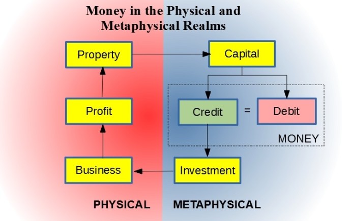
Another concept to keep in mind is Hernando de Soto’s (2000) epiphany that a house is just a shelter from the weather until it is secured by a property title. He envisioned that such things as titles inhabit what amounts to a separate universe parallel to the physical universe where the house resides. Borrowing a term from philosophy, one might call this a metaphysical universe made up of metadata that describes objects in the physical universe. de Soto’s idea was that existence of the property-title metadata turns the house into wealth that can become capital through the agency of beneficial ownership.
If one has beneficial ownership of a property title, one can encumber it by, for example, using it to secure a loan. One can then invest the funds derived from that loan into increased productive capacity of a business–back in the physical universe. Thus, the physical house is just an object, whereas the property title is capital (de Soto, 2000). It is the metaphysical capital that is transferable, not the physical property. In the transaction between the farmer and the herdsman above, what occurred was a swap between the two parties of de-Sotoan capital derived from beneficial ownership of the cattle and of the daughter, and it happened in the metaphysical universe.
What Is Money, Really?
Much of the confusion about forex rates arises from conflating capital and money. Masi (2019) speculated that money in circulation (e.g., M1) captures only half of what money really is. Borrowing concepts from both physics and double-entry bookkeeping, he equated money with a two-part conserved quantity he referred to as credit/debit. (Note that here the words “credit” and “debit” are not used strictly according to their bookkeeping definitions.) Credit arises in tandem with creation of an equal amount of debit. Thus, the net amount of money (equaling credit-minus-debit) is always the same: zero. A homeowner raising funds through a home-equity line of credit (HELOC) does not affect his or her total wealth. The transaction creates funds (credit) and debt (debit) in equal amounts. Similarly, a government putting money into circulation, whether by printing pieces of paper, or by making entries in a digital ledger, automatically increases the national debt.
Capital, on the other hand, arises, as de Soto (2000) explained, as metadata associated with property. The confusion comes from the fact that both capital and money are necessarily measured in the same units. While capital can increase through, say, building a house, or it can decrease by, for example, burning a house down, the amount of money (as credit/debit) can never change. It’s always a net zero.
The figure above shows how de Soto’s (2000) and Masi’s (2019) ideas combine. The cycle begins on the physical side with beneficial ownership of some property. On the metaphysical side, that beneficial ownership is represented by capital (i.e., property title). That capital can be used to secure a loan, which creates credit and debit in equal amounts. The beneficial owner is then free to invest the credit in beneficial ownership of a productive business back on the physical side. The business generates profits (e.g., inventory) that the owner retains as an increase in property.
The debit that was created along the way stays on the metaphysical side as an encumbrance on the total capital. The system is limited by the quantity of capital that can be encumbered, which limits the credit that can be created to fund continuing operations. The system grows through productivity of the business, which increases the property that can be represented by new capital, which can be encumbered by additional credit/debit creation, which can then fund more investment, and so forth. Note that the figure ignores, for simplicity, ongoing investment required to maintain the productive assets, and interest payments to service the debt.
Wang’s mismanagement strategy amounted to deficit spending–using a printing press to create credit/debit faster than the economy can generate profit to be turned into an increasing stock of capital (Onge, 2017). Eventually, the debt level rises to encumber the entire capital supply, at which point no new credit/debit can be created. Continued running of Wang’s printing press merely creates more fiat money to chase the same amount of goods: inflation. Thus, inflation arises from having the ratio of money creation divided by capital creation greater than one.
In Song China, investment collapsed due to emphasis on rent seeking, followed by collapsing productivity (Onge, 2017). Hyperinflation set in as the government cranked the printing presses just to cover national-debt service. Finally, hungry outsiders, seeing the situation, swooped in to seize the remaining productive assets. First it was the Jurchens, then the Mongols.
Forex and Hyperinflation
The Song Chinese quickly saw Wang’s mismanagement at work, and kicked him out of office (Onge, 2017). They, however, failed to correct the practices he’d introduced. Onge (2017) pointed out that China’s GDP per person at the start of the Song dynasty was greater than that of 21st-century Great Britain. Under Wang’s policies, decline set in around 1070–80, and GDP per person had fallen by 23% by 1120. Population growth changed to decline. Productivity cratered. Inflation turned to hyperinflation. The Jurchen, without the burden of Wang’s teachings, were slower to inflate their currency.
As Chinese inflation increased relative to that of the Jurchen, exchange rates between Jurchen and Chinese currencies changed rapidly. The Jurchen fiat currency became stronger relative to that of the Chinese. This tale illustrates how changes in forex rates follow relative inflation between currencies, and argues for using the interest rate approach to predict future equilibrium forex rates (Scott Hacker, et al., 2012).
Conclusion
Forex rates are free to fluctuate because money is neutral (Patinkin & Steiger, 1989). Viewing money as a conserved two-fluid metaphysical quantity (Masi, 2019) shows how a country’s supply of de-Sotoan capital constrains the money supply, and shows how an economy grows through profits from productive businesses (de Soto, 2000). It also explains inflation as an attempt to increase the money supply faster than the capital supply can grow. The mismatch of relative inflation affects equilibrium forex rates by increasing strength of one currency relative to another, and argues for the interest-rate approach to forex theory (Scott Hacker, et al., 2012).
References
de Soto, H. (2000). The mystery of capital. New York, NY: Basic Books.
Masi, C. G. (2019, June 19). The Fluidity of Money. [Web log post]. Retrieved from http://cgmblog.com/2019/06/19/the-fluidity-of-money/
Onge, P. S. T. (2017). How paper money led to the Mongol conquest: Money and the collapse of Song China. The Independent Review, 22(2), 223-243.
Patinkin, D., & Steiger, O. (1989). In search of the “veil of money” and the “neutrality of money”: A note on the origin of terms. Scandinavian Journal of Economics, 91(1), 131.
Scott Hacker, R., Karlsson, H. K., & Månsson, K. (2012). The relationship between exchange rates and interest rate differentials: A wavelet approach. World Economy, 35(9), 1162–1185.
West, M. L. [Ed.] (2008). Hesiod: Theogony and works and days. Oxford, UK; Oxford University Press.
The government-funded project to develop Polaris, the first submarine-launched ICBM, transformed the way projects – and indeed most 21st-century businesses – are run. Image by Alexyz3d/Shutterstock
9 February 2020 – I’m about half way through a course on global economics at Keiser University, and one of this week’s assigned readings is a 2012 article by Argentine-American legal scholar Fernando R. Tesón discussing his views on the ethical basis of free trade. I was particularly struck by the wording of his conclusion section:
More often, trade barriers allow governments to transfer resources in favor of rent-seekers and other political parasites. … Developed countries deserve scorn for not opening their markets to products made by the world’s poor by protecting their inefficient industries, while ruling elites in developing nations deserve scorn for allowing bad institutions, including misguided protectionism. (p. 126)
This was unusually blunt in a scholarly article! Tesón, however, did a good job of making his case. Citing David Ricardo’s and Hecksher-Olin’s theories of comparative-advantage, He provided a well-thought-out, if impassioned, argument that trade barriers are misguided at best, and at worst unconscionable. Among the practices he heaped scorn upon are “tariffs, import licenses, export licenses, import quotas, subsidies [emphasis added], government procurement rules, sanitary rules, voluntary export restraints, local content requirements, national security requirements, and embargoes” (Tesón, 2012, p. 126).
Generally, that was a defensible list. All of those practices tend to slew market-based purchase decisions toward goods produced by firms lacking true competitive advantage. The case against subsidies, however, is not so simple. There are various reasons for creating subsidies and ways of applying them. Not all are counterproductive from an economic-development standpoint.
Stephen Redding, in a 1999 article entitled “Dynamic comparative advantage and the welfare effects of trade” pointed out that comparative advantage is actually a dynamic thing. That is, it varies with time, and producers can, through appropriate investments, artificially create comparative advantages that are every bit as real as the comparative-advantage endowments that the earlier theorists described.
The original Ricardian model envisioned countries endowed with innate comparative advantages for producing some good(s) relative to producing the same good(s) in another country (Kang, 2018). Redding pointed out that a country’s productivity for manufacturing some good increases with time (experience) spent producing it. He posited that if the country’s competitors’ comparative advantage for producing that good is not great, it may be possible for the country to, through investing in or subsidizing development of an improved production process, overtake its competitors. In this way, Redding asserted, the relative competitive advantage/disadvantage situation may be reversed.
The counterargument to subsidizing such a project is that the subsidy has an opportunity cost in that the subsidy uses funds exacted from the country’s taxpayers to benefit one or more selected firms. Tesón’s position is that this would be an inappropriate use of taxpayer funds to benefit only a small subset of the country’s citizens. This is ipso facto unfair, hence his stigmatizing such a decision. The reductio ad absurdum rejoinder to this argument is that it leaves government powerless to effect economic development.
In a democracy, government decisions are assumed to have tacit acceptance by the whole population. Thus, an action by the government to support a small group developing a comparative advantage through a subsidy must be assumed to have a positive externality for the whole population.
If the government is an autocracy or oligarchy, there is no legitimate claim to fairness for any of its decisions, anyway, so the unfairness argument is moot.
There are thus conditions under which subsidizing firms or industries to develop enhanced productive capacity for some good make economic sense. Those conditions are as follows:
Competitors’ comparative advantage is small enough that it can be overcome with a reasonable subsidy over a reasonable length of time;
There is reason to expect the country will be able to maintain its improved comparative advantage situation after subsidies have been removed;
Achieving a comparative advantage for production of that good will have ripple effects that will generate comparative advantage throughout the economy.
If and only if all of these conditions obtain is it reasonable to create a temporary subsidy.
An example of an inappropriate subsidy is that by the European Union for Airbus, which began with the company’s launch in 1970 to create an EU-based large civil aircraft (LCA) industry to compete with the U.S.-based Boeing Aircraft Company and continues today (European Commission, 6 October 2004). While this history indicates that item 1 on the list above was fulfilled (Airbus became an effective competitor for Boeing in the 1980s), and item 3 certainly was fulfilled, the fact that the subsidies continue today, half a century later, indicates that item 2 was not fulfilled.
On the other hand, the myriad salutary effects that came out of the Polaris missile program of the mid-20th Century shows that all three conditions were valid for that government-subsidized project (Engwall, 2012).
References
Engwall, M. (2012). PERT, Polaris, and the Realities of Project Execution. International Journal of Managing Projects in Business,.5(4), 595-616.
European Commission. (6 October 2004). EU – US Agreement on Large Civil Aircraft 1992: key facts and figures. (MEMO/04/232). Retrieved from https://ec.europa.eu/commission/presscorner/detail/en/MEMO_04_232
Kang, M. (2018). Comparative advantage and strategic specialization. Review of International Economics, 26(1), 1–19.
Redding, S. (1999). Dynamic comparative advantage and the welfare effects of trade. Oxford Economic Papers, 51, 15-39.
Tesón, F.,R. (2012). Why free trade is required by justice. Social Philosophy & Policy, 29(1), 126-153.
Shanghai, China is the epicenter of the Chinese Miracle. Image by f11photo/Shutterstock
14 December 2019 – The following essay is a verbatim copy of one I recently posted to a Global Business discussion site in response to a link emailed to me by Dr. Tiffany Jordan of Keiser University.
Thank you, TJ, for sending along a link to Steve Sjuggerud’s documentary on Chinese development. History teaches us that 5,000 years ago, China was one of two (maybe three, if you count Central America) population centers (the other was Egypt) where folks independently invented civilization. You can’t go far wrong by betting on people that smart!
The second factor in this story is that one out of six human beings on this planet is Chinese. With that many really smart people let loose to work together, they’re bound to push the limits of economic development. The last time that happened anywhere was in the 18th century when steam technology was let loose among the newly liberated populations of England, North America, and Europe. The resulting Industrial Revolution was a similar game changer. People from the countryside flocked to the cities to make the most of revolutionary technology, and made vast piles of wealth in the process. Sound familiar?
So, what could go wrong? The known preference of the Chinese people for long power distance is what could go wrong (Hofstede, 1993). Since Qin Shi Huang patched together the Chinese Empire in 221 BCE (Shi, 2014), the country has had a nearly unbroken record of authoritarian rule, which is why, after all this time, they’re still stuck with “emerging nation” status. The latest period of lax central control started in the mid-1970s, when Mao Zedong lost control of his Marxist People’s Republic (PRC), and good things started happening in China.
China is home to two philosophies at opposing ends of the power-distance spectrum: Taoist egalitarianism and Confucian formality (Carnogurská, 2014). Taoists insist (among other things) on individual self-rule. Confucionists insist on respect for authority (Zhou, 2011). You can guess which philosophy Xi Jinping’s power-grabbing PRC favors! It is no accident that the slowing of China’s economic expansion immediately followed Xi’s re-institution of central authority. The stark contrast can be seen in the difference between the miracle on the Chinese mainland and the even-bigger miracle that has been playing out in Hong Kong.
I’m always ambivalent, however, about investing in the Chinese “miracle.” Back in the early 1990s I was asked to duplicate my success helping expand an American electronics publication into Europe by doing the same thing in China. With images from Tiananmen-Square events fresh in my mind, I declined. Unlike my corporate bosses, I just didn’t trust the PRC leadership to play nice. That corporation is now out of the publishing business! I’d done the same thing in the 1970s when I declined the last Shah of Iran’s invitation to take our Boston-based Physics Department to Tehran University–just before theirrevolution broke out. (Whew!)
China is not Iran, and Xi Jinping is not Mohammad Reza Shah. Pres. Xi likes leading the fastest-growing economy on the planet, but is facing his big test with current events in Hong Kong. Will he figure a way to defuse that uprising, or will his unenlightened cronies in Beijing push him into a disasterous reprise of Tiananmen-Square? I’m not jumping onto the Chinese bandwagon until I see the result.
References
Carnogurská, M. (2014). Xunzi, an ingeniously critical synthesist of Chinese philosophy of the pre-Qin period. Journal of Sino – Western Communications, 6(1), 3-25.
Hofstede, G. (1993). Cultural constraints in management theories. Executive, 7(1), 81–94.
Shi, J. (2014). Incorporating all for one: The first emperor’s tomb mound. Early China, 37(1), 359-391.
Zhou, H. (2011). Confucianism and the legalism: A model of the national strategy of governance in ancient China. Frontiers of Economics in China, 6(4), 616-637.
A temporal framework to understand team dynamics with high resolution. Image by Klonek et al
30 October 2019 – The essay below was posted to the Keiser University DBA 710 Week 8 Discussion Forum. It is reproduced here in the hope that readers of this blog will find this peek into state-of-the-art management research interesting.
This posting is a bit off topic for Week 8, but it reviews a paper that didn’t cross my desk in time to be included in last week’s discussions, where it would have been more appropriate. In fact, the copy of the paper I received was a manuscript version of a paper accepted by the journal Organizational Psychology Review that is at the printer now.
The paper, written by an Australian-German team, covers recent developments in measuring variables apropos management of decision teams in various situations (Klonek, Gerpott, Lehmann-Willenbrock & Parker, in press). As we saw last week, there is a lot of work to be done on metrology of leadership and management variables. The two main metrology-tool classifications are case studies (Pettigrew, 1990) and surveys (Osei-Kyei & Chan, 2018). Both involve time lags that make capturing data in real time and assuring its freedom from bias impossible (Klonek, Gerpott, Lehmann-Willenbrock & Parker, in press). Decision teams, however, present a dynamic environment where decision-making processes evolve over time (Lu, Gao & Szymanski, 2019). To adequately study such processes requires making time resolved measurements quickly enough to follow these dynamic changes.
Recent technological advances change that situation. Wireless sensor systems backed by advanced data-acquisition software make in possible to unobtrusively monitor team members’ activities in real time (Klonek, Gerpott, Lehmann-Willenbrock & Parker, in press). The paper describes how management scholars can use these tools to capture useful information for making and testing management theories. It provides a step-by-step breakdown of the methodology, including determining the appropriate time-resolution target, choosing among available metrology tools, capturing data, organizing data, and interpreting data. It covers working on time scales from milliseconds to months, and mixed time scales. Altogether, the paper provides invaluable information for anyone intending to link management theory and management practice in an empirical way (Bartunek, 2011).
References
Bartunek, J. M. (2011). What has happened to Mode 2? British Journal of Management, 22(3), 555–558.
Klonek, F.E., Gerpott, F., Lehmann-Willenbrock, N., & Parker, S. (in press). Time to go wild: How to conceptualize and measure process dynamics in real teams with high resolution? Organizational Psychology Review.
Lu, X., Gao, J. & Szymanski, B. (2019) The evolution of polarization in the legislative branch of government. Journal of the Royal Society Interface, 16: 20190010.
Osei-Kyei, R., & Chan, A. (2018). Evaluating the project success index of public-private partnership projects in Hong Kong. Construction Innovation, 18(3), 371-391.
Pettigrew, A. M. (1990). Longitudinal Field Research on Change: Theory and Practice. Organization Science, 1(3), 267–292.